Definition
Stochastic calculus is a way to conduct regular calculus when there is a random element.
Regular calculus is the study of how things change and the rate at which they change.
Description
Think of stochastic calculus as the analysis of regular calculus + randomness.
Regular Calculus
Regular calculus studies the rate at which things changes.
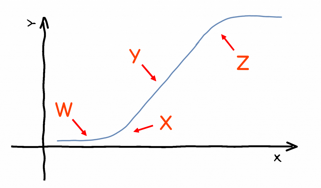
- At W, there is 0 change
- At X, there is an increasing increase
- At Y, there is a constant increase
- At Z, there is a decreasing increase
The red lines indicate the rate of increase at the black dots.
As the red lines become steeper, the increase in values is going up at a faster pace.
Imagine that we are climbing up a ladder, but now we are climbing up at a faster pace.
Randomness
Let’s talk about randomness before combining this with the earlier section on regular calculus.
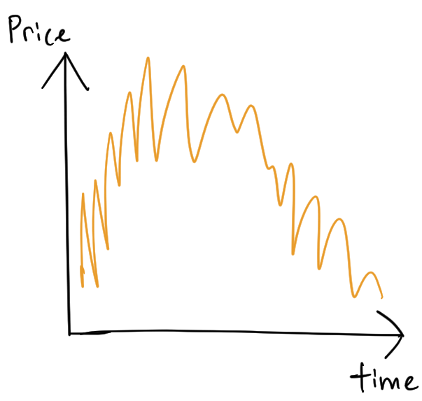
This is what a bunch of random charts look like:
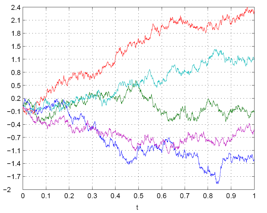
This behavior is described as Brownian motion.
This means that their behaviour is random, but over the long run and with enough samples, their overall movement resembles a bell shape. In other words, they are normally distributed.
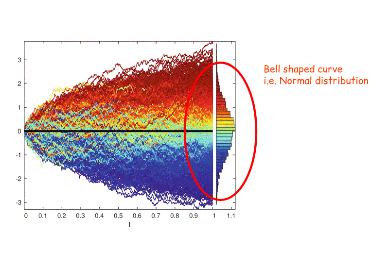
This randomness is not so random after all. The end result of all these random movements is a bell shaped output. (See the bell shape by tilting your head to the right.)
That means that most of the data points end in the middle while the rest are spread out across the sides.
More info on Normal Distribution: Normal Distribution – MathIsFun
In Brownian motion, the values can be negative. However, stock prices can’t be negative.
Thus, in finance, we use geometric Brownian motion to model our stock prices.
Geometric Brownian motion (GBM) is essentially regular Brownian motion but with an upward drift.
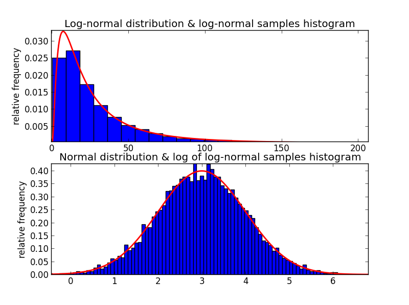
The end result of all these GBM movements is a skewed bell shaped output.
This skewed bell-shaped curve no longer resembles a normal distribution. It now resembles a log-normal distribution.
Stochastic Calculus = Regular Calculus + Randomness
When we zoom in on a curve chart, we get a nice curve line. We can then measure the rate of increase using those slopes.
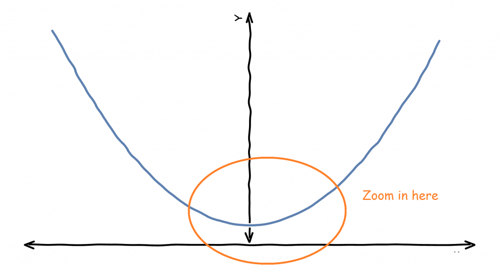
The curve is smooth
Now let’s look at a chart with randomness.
If we zoom in, we see that it looks… somewhat the same.
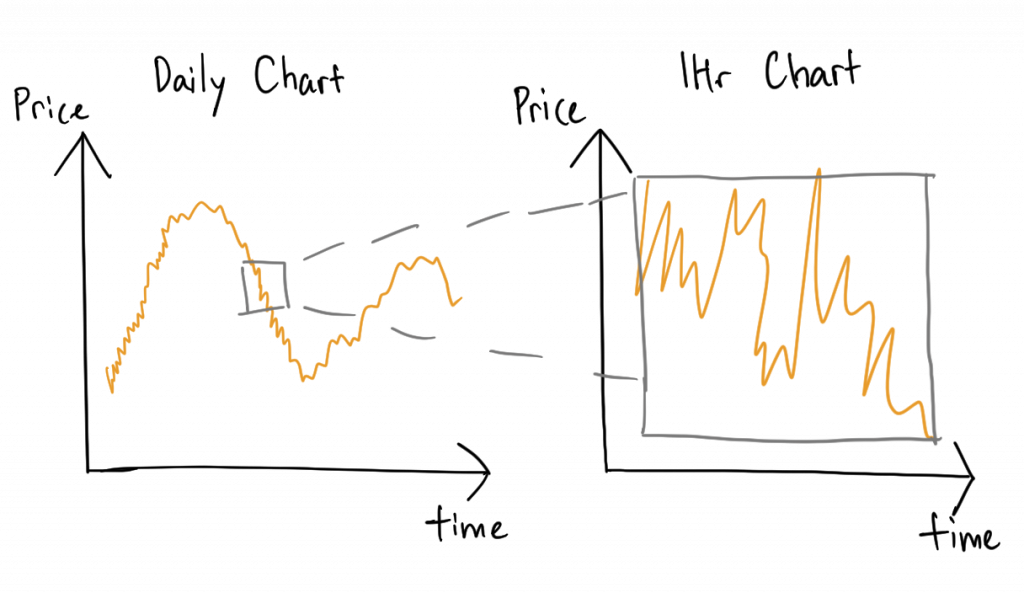
We can keep zooming in but we will not be able to find a smooth curve. Without a smooth curve, we can’t draw those slope lines productively.
Thus, normal calculus will fail here. This is why we need stochastic calculus.
Stochastic Calculus Mathematics
The main aspects of stochastic calculus revolve around Itô calculus, named after Kiyoshi Itô.
The main equation in Itô calculus is Itô’s lemma. This equation takes into account Brownian motion.
Itô’s lemma:
![\[ dX_t = \mu_t dt + \sigma dB_t\]](https://algotrading101.com/wiki/wp-content/ql-cache/quicklatex.com-0d00a1995fa042ff7cbd81b570bbf5bb_l3.png "Rendered by QuickLaTeX.com")
Explanation: Change in X = Constant A * change in time + Constant B * change due to randomness as modeled by Brownian motion.
Which means the change in the value of a variable = some constant value over time + change due to randomness multiplied by another constant.
More info on the derivation of Itô’s lemma: Derivation of Itô’s lemma by Math Partner
A variation of Itô’s lemma that uses GBM is:
![\[ dX_t = \mu_t X_t dt + \sigma X_t dB_t\]](https://algotrading101.com/wiki/wp-content/ql-cache/quicklatex.com-f149fe3580e64a44b2cd0b1811bd4356_l3.png "Rendered by QuickLaTeX.com")
Before we explain it. Let’s replace X (a regular variable) with S (stock price) so that you can visualize this better.
![\[ dS_t = \mu_t S_t dt + \sigma S_t dB_t\]](https://algotrading101.com/wiki/wp-content/ql-cache/quicklatex.com-551ceeb90a58881b0acfb916cee6b471_l3.png "Rendered by QuickLaTeX.com")
In this case, we try to link the equation to finance. Let S be stock price.
Explanation: Change in S = Constant A * Current S * change in time + Constant B * Current S * change due to randomness as modeled by GBM
Which means the change in the stock price = current stock price multiplied by some constant value over time +
current stock price + change due to randomness multiplied by another constant.
That should intuitively make sense as over time, the change of the stock price is based on some overall trend (the Constant A part) and an element of randomness (the Constant B part and randomness part).
Constant A and Constant B are usually derived by analyzing historical market data.
Finance and Stochastic Calculus
This is where we relate everything we’ve just said to finance.
In 1900, Louis Bachelier, a mathematician, first introduced the idea of using geometric Brownian motion (GBM) on stock prices.
His theory is later built upon by Robert Merton and Paul Samuelson in their work on options pricing. They won an Nobel Prize in Economics for it.
Essentially, these mathematicians argue that GBM can be used to model stock prices because it is said that:
- The GBM process has only positive values. Stock prices only has positive values.
- Expected value of the data in the next time period has nothing to do with the last time period. Similarly, it is said that the expected value of the stock price in the next time period has nothing to do with the last time period
- The GBM chart is rough and random. Stock prices look rough and random.
- Calculations with GBM processes are relatively easy
However, those points above are debatable.
- In reality, the randomness and volatility changes over time. In GBM, the volatility is assumed to be constant.
- In reality, there are sudden jumps in prices. In GBM, there are not.
- In reality, the stock prices may not be random and log-normally distributed in the long run. In GBM, they are.
Stochastic calculus as applied to finance, is a form of pseudo science. There are assumptions that may not hold in real-life. Some of the assumptions are there for the convenience of mathematical modelling.
Black Scholes Model – Application to Finance
The most famous application of stochastic calculus to finance is to price options (options are a special financial instrument that gives the holder the choice to buy or sell an asset at a certain price).
The main intuition is that the price of an option is the cost of hedging it.
By hedging, we mean that we can separately create a combination of stocks and cash to mimic the market exposure of the option.
Thus, the cost of this hedging process should be the price that option is worth.
Price of option = cost of hedging with stock and cash.
Now, we can calculate the price of the option if we assume that the stock can be modeled using Ito’s lemma, which brings us back to the equation above:
Using the above equation and the fact that the price of the option = cost of hedging with stock and cash, we can derive our Black-Scholes equation
Black-Scholes Equation
![\[ \frac{\partial V}{\partial t} + \frac{1}{2}\sigma^2 S^2 \frac{\partial^2 V}{\partial S^2} + rS\frac{\partial V}{\partial S} - rV = 0 \]](https://algotrading101.com/wiki/wp-content/ql-cache/quicklatex.com-46952bfac796fef247258ec7bd73dda3_l3.png "Rendered by QuickLaTeX.com")
We are not going to do the derivation here as it is too technical.
Here is the derivation: Paul Wilmott on Quantitative Finance, Chapter 5, Black-Scholes
Once you solve that equation and turn it into a form that we can plug in figures and use, you’ll get the Black-Scholes Formula:
![\[ \mathrm C(\mathrm S,\mathrm t)= \mathrm N(\mathrm d_1)\mathrm S - \mathrm N(\mathrm d_2) \mathrm K \mathrm e^{-rt} \label{eq:2} \]](https://algotrading101.com/wiki/wp-content/ql-cache/quicklatex.com-43719260ed158f44596dbce2e119cf8a_l3.png "Rendered by QuickLaTeX.com")
![\[ \hspace*{-10cm} \text{where} \]](https://algotrading101.com/wiki/wp-content/ql-cache/quicklatex.com-ea92420ebc61e426daffcc05de4ddf3d_l3.png "Rendered by QuickLaTeX.com")
![\[ \mathrm d_1= \frac{1}{\sigma \sqrt{\mathrm t}} \left[\ln{\left(\frac{S}{K}\right)} + t\left(r + \frac{\sigma^2}{2} \right) \right] \]](https://algotrading101.com/wiki/wp-content/ql-cache/quicklatex.com-e57df4ec39972564fde137703cc70881_l3.png "Rendered by QuickLaTeX.com")
![\[ \mathrm d_2= \frac{1}{\sigma \sqrt{\mathrm t}} \left[\ln{\left(\frac{S}{K}\right)} + t\left(r - \frac{\sigma^2}{2} \right) \right] \]](https://algotrading101.com/wiki/wp-content/ql-cache/quicklatex.com-8fbc37f530b04d6f1e69db78f04ac39f_l3.png "Rendered by QuickLaTeX.com")
![\[ N(x)=\frac{1}{\sqrt{2\pi}} \int_{-\infty}^{x} \mathrm e^{-\frac{1}{2}z^2} dz \label{eq:5} \]](https://algotrading101.com/wiki/wp-content/ql-cache/quicklatex.com-7c1836482af0d7ed9e06af2f29481525_l3.png "Rendered by QuickLaTeX.com")
This is how you get from the equation to the formula:
Solution of the Black-Scholes Equation – University of Nebraska (warning: It gets technical)
Links to Other Explanations
- Outline of Stochastic Calculus (Video) – Maths Partner
- Geometric Brownian Motion – Wikipedia
- Black-Scholes Model – Wikipedia
- Black-Scholes Equation – Wikipedia
Related Terms